SUMPRODUCT function in Excel returns the sum of the products of the corresponding ranges or arrays. Let’s check the syntax for this function.

Formula Syntax: SUMPRODUCT (array 1, [array 2], [array 3], …)

The arrays in the formula are the ranges of the cells that we wish to multiply.

SUMPRODUCT function in Excel:

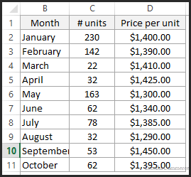
Let’s take an example, we have a data with number of units sold and the price per unit from January to October as shown in the image below. We would like to find out the total revenue generated for the above said months. Instead of doing individual product calculation and summing it up, we can easily calculate by using SUMPRODUCT function in excel.

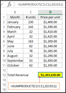
To find out the total revenue generated we put “=SUMPRODUCT(C2:C11,D2:D11)” as shown in the image below.

Here, in the formula, ‘C2:C11’ is the array 1 and array 2 is ‘D2:D11’. These two arrays in the SUMPRODUCT function give us the total revenue.

SUMPRODUCT function using BOOLEAN expression:

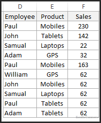
Now, let’s take an example to understand how SUMPRODUCT function in excel works with BOOLEAN expression. Assume we have sales data of employees, for products like Mobiles, Tablets, and Laptops etc. as shown in the image below.

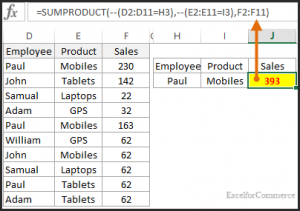
As we are interested in calculating how many units of Mobiles were sold by the Employee with the name Paul. Enter ‘Paul’ or select Paul from dropdown list as Employee name in the cell (H3), Product name as ‘Mobiles’ in the cell (I3) and put the following formula in the cell (J3) “=SUMPRODUCT(–(D2:D11=H3),–(E2:E11=I3),F2:F11)” as shown in the image below.

Here, ‘D2:D11’ is the Employee name range to which we are comparing the employee name entered/ selected in the cell ‘H3’. ‘E2:E11’ is the Product range to which we are comparing the product name entered/ selected in the cell ‘I3’ and then finally ‘F2:F11’ is the range which returns the sales figures. As we can see from the above example, ‘Paul’ sold ‘393’ mobile units in total.

If you have observed the formula used carefully, we used double hyphens (–) before arrays/lists. These hyphens convert the list of Boolean values to zeros and ones. One hyphen is to negate the values to numbers and reverse the sign. So, TRUE turns into -1 and FALSE turns into 0. The second hyphen is to reverse the sign and to convert it into actual number (i.e. 1 for TRUE and 0 for FALSE).

This is how we use SUMPRODUCT function in Excel. For more queries, feel free to contact our Excel Expert here.