
- 01Jan2015
-
How to sort horizontally in Excel? (from left to right)
Sorting horizontally in Excel:
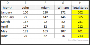
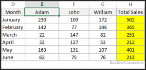
Sorting horizontally in excel (from left to right) is required when we have a table/data as shown in the image below. In the below image, we want to sort horizontally based on employee name. This blog explains how to sort multiple columns horizontally from left to right. Let’s take a sample data where we have employees with the name John, Adam and William with their sales figures for the months January to June. As we can see in the image below, the table is not sorted alphabetically by the employee names.
Where can I find Sort option?
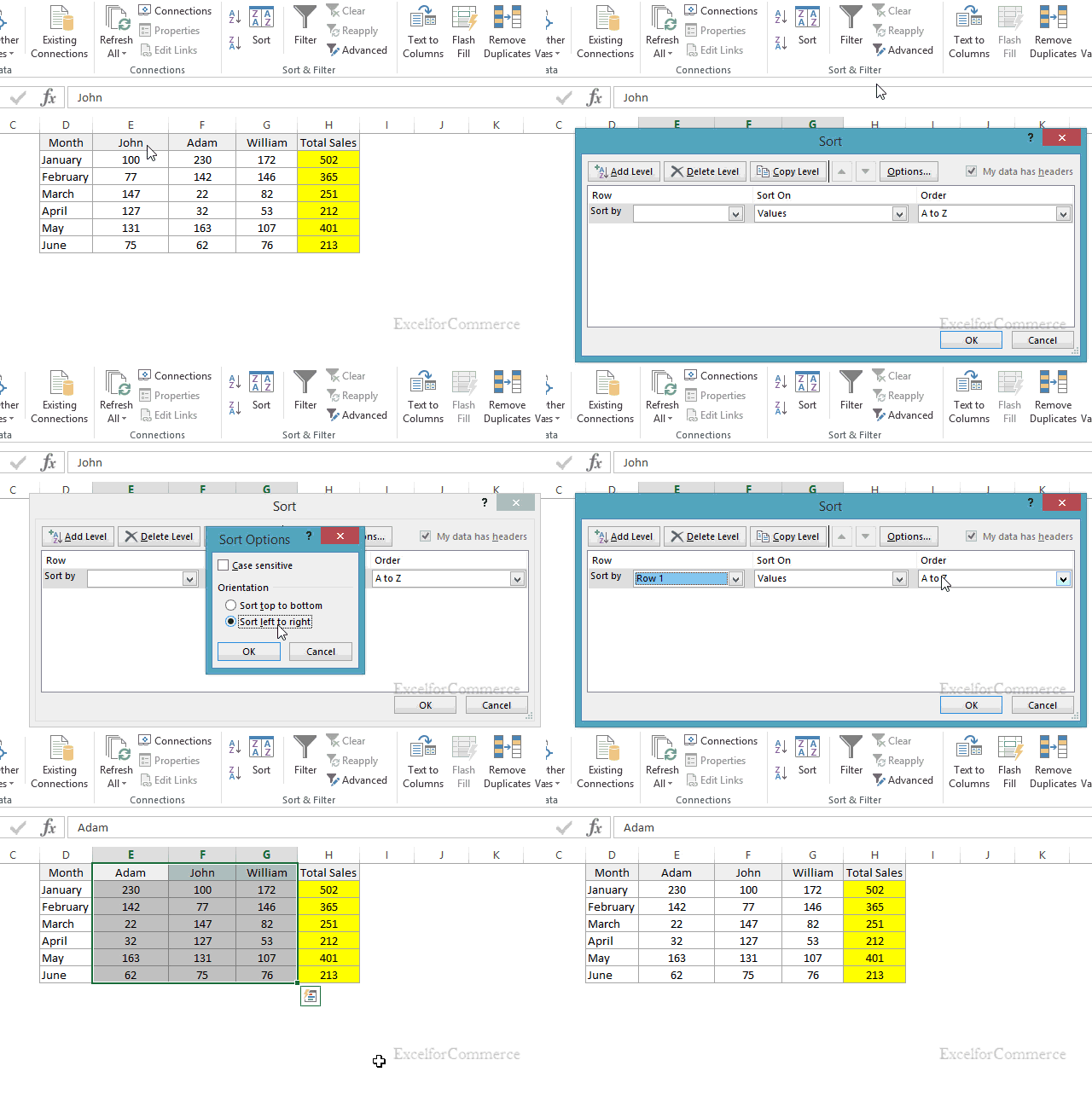
Sort option is available in Sort and Filter section in Data tab in Excel ribbon as shown in the image below.
Below are the steps to sort the data
Step 1: Select Data/ Range to sort
Step 1a:
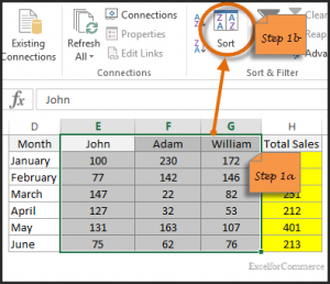
Here in the data, month column and Total Sales column are not required to sort. The main objective is to sort all the employee columns. To do this, we select the range as shown below (E1:G7)
Step 1b:
Click on sort from the Excel ribbon.
Step 2: Sorting the table
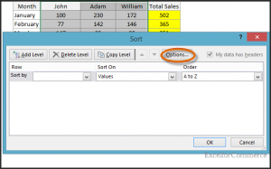
After clicking on Sort, we get a pop up window with options as shown in the image below. Now, click on options in that window.
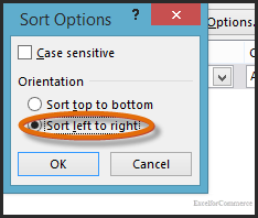
Now, we get another window (sort options) where we need to select sort left to right and then click OK
Now, we are back to the previous window. Here we need to select Sort by ‘Row 1’ from the dropdown list as we need to sort the employee names alphabetically. Order must be in A to Z for sorting. After making these selections, click ok.
Now the table is sorted horizontally from left to right and the final table looks like the image shown below.
This is how we Sort horizontally in Excel. If you still have any questions, feel free to contact us here.
- 1 Jan, 2015
- Excel for Commerce
- 0 Comments
- Excel Consultant, Excel Expert, Sort horizontally in Excel,



Comments