In our day to day lives, at an individual level or at a business level, we come across questions like:

• “How much should my personal expenses on a particular item be cut down so that my total expenses don’t reach the threshold?”
• “To what extent should the company increase its advertising spend so that revenue is maximized? “
• “How much should I invest in a particular fund so that I get a final amount of $100,000 at the end of 5 years?”

Excel provides a very powerful tool or add-in called “Solver” that answers all these questions.  Without stretching a lot many of your mental muscles, you can use Solver to solve your problems. It comes up with solutions by performing various permutations and combinations and simplifies your work.

Setting up Solver in Excel

• Click on the “File” or the “Office Button” on your ribbon. You will find “Options” button from which select “Add-Ins”. It displays a list of different add-ins within excel. Choose the “Solver Add-In” and click “Go”.

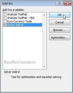
• The Add-ins box pops up and the “Solver Add-in“ must be selected which adds solver to ribbon . Click “OK” after selecting .

• The “Solver” add-in can now be seen in “Analysis” group within “Data” tab of the excel ribbon.

Once the solver add-in is added, you are good to go. You can use it to solve various problems.

Case-study 1:

Let us solve a simple sum of two variables ‘a’ & ‘b’ using solver

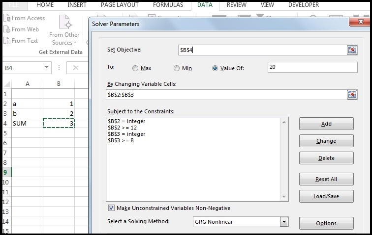
• Values of “a” and “b” are placed in B2 & B3 cells. The sum is placed in B4 which is “=Sum(B2:B3) “
• Initially let us give the values of 1 & 2 to ‘a’ & ‘b’ and the sum is derived as 3 in cell B4. This will enable the solver to understand the logic in cell B4 (sum of B2 & B3 here) and it makes sure to use the same logic to come up with the solution.
• Now, let us click on the Solver tool to find out what the values of “a” and “b” must be, so that we get a desired result of say 20.

• We can see that the “Solver Parameters” box pops up.
• Here the “Set Objective” is $B$4 where the output or sum of two variables is calculated. – Since we are not looking at a Min or Max value but a fixed output value of 20, “Value of” radio button should be selected and output value of 20 is entered.
• “By Changing variable cells” option indicates the variables in our example which are “a” & “b” and their reference is given as “$B$2:$B$3”.
• Solver also allows you to give your constraints, which are supposed to be followed by the values according to you. In this example, the constraints are given as:
  • B2 & B3 are integers
  • B2 must be greater than or equal to 12
  • B3 is greater than or equal to 8
• Once your desired ranges and constraints are included, Click on “Solve” button.

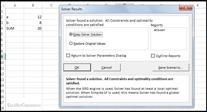
• You can notice that the values in B2 and B3 are updated with solver results and the same has happened with their corresponding sum in B4.
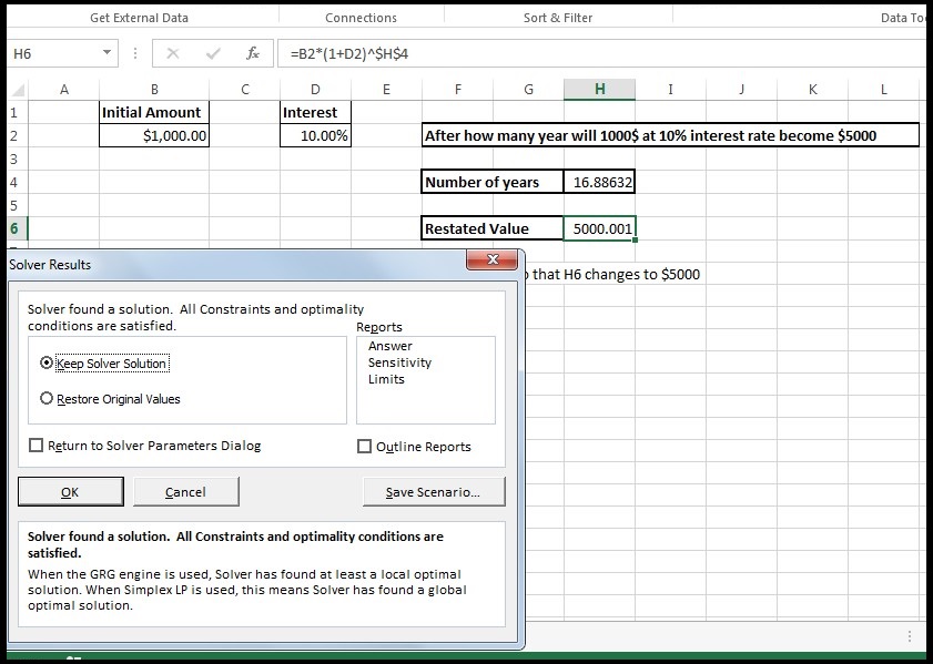
•  You also have an option to “Keep Solver Solution” or “Restore Original Values” in “Solver Results” pop-up. This pop-up is shown immediately after the solver comes up with the solution.

Case-study 2:

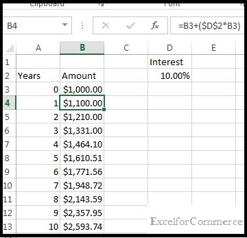
Let us say, you lent an amount of $1,000 at an interest rate of 10% and the final amount compounds to $2,593.74 after 10 years of time.

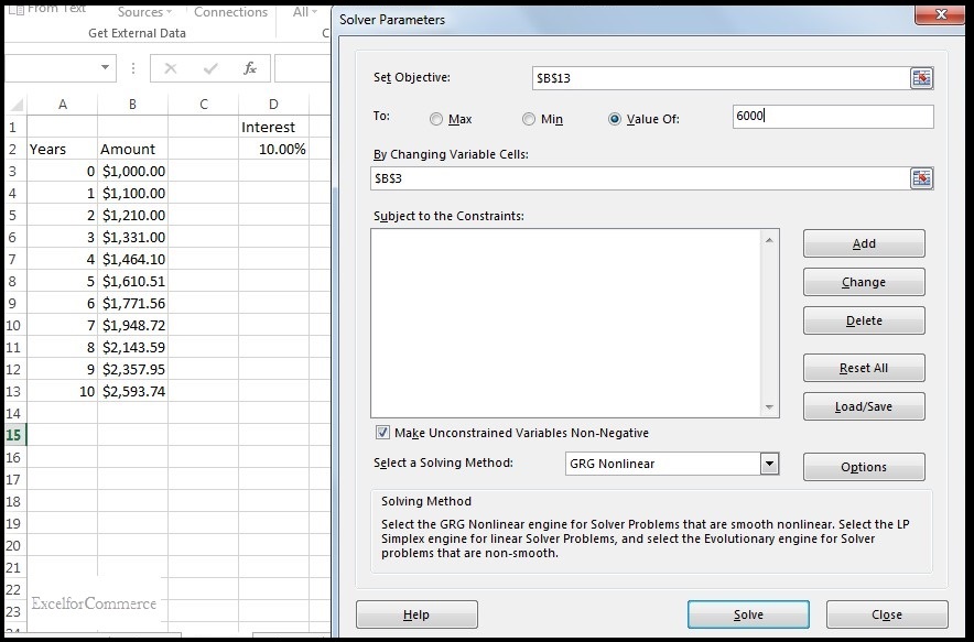
We want to know how much should be lent as an initial amount at 10% interest rate for a period of 10 years so that at the end of 10^th year, the total amounts sums up to $6,000.

Let’s use Solver to solve this problem

• Here, the “Set Objective:” is the Final Amount cell “B13” which is set to value of $6,000.
• The Initial amount is what we are trying to find out, so the cell “B3” is entered in “By changing variable cells:” and Click on ‘Solve”.

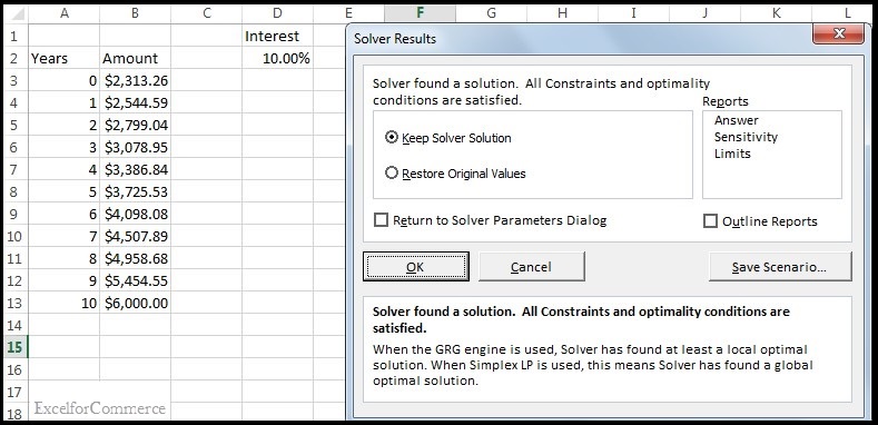
As you can observe, Solver has come up with a solution satisfying all conditions and the values in the Amount column are updated with solver results. In Summary, the initial amount has to be $2,313.26 so that the final amount is compounded to $6000 after 10 years.

Case-study 3:

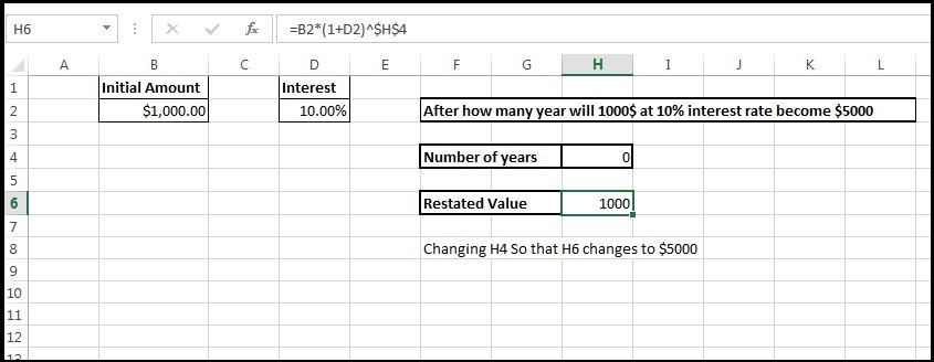
Taking the same example – now, let us find out the number of years it will take for the same initial amount of $1,000 to sum up to $5,000 at an interest rate of 10%.

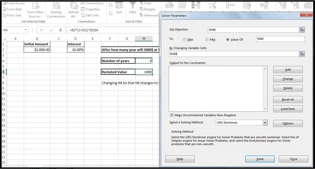
• The formula used in the previous problem does not take “years” into consideration and if used in the present case too, the solver will misinterpret the logic and will not predict the desired values.  So, the formula in cell H6 displaying the compounded amount after 10 years has to be “B3*(1+D2)^$H$4” where $H$4 is “Number of years”.
• Now, let’s observe how solver works out the solution for this problem

• The “Set Objective” here is H6 which must be target output value of $5,000 by changing the variable cell “H4” i.e. Number of years.
• After setting all the parameters, click “Solve” button.

We observe that Solver has done its part by predicting the ‘Number of years’ that takes to arrive at a final amount of $5,000 as 16.88632 and the results are updated in respective cells accordingly.

Isn’t using solver easy and effort reducing? Start using it to make quick decisions with great accuracy. If you have any questions on Solver, feel free to contact us at excelexpert@excelforcommerce.com.